Photometry ✨#
After an observation is done, a common need is to reduce and extract fluxes from raw FITS images.
In this tutorial you will learn how to process a complete night of raw data from any telescope with some basic reduction tools provided by prose.
Example data#
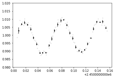
You can follow this tutorial on your own data or generate a synthetic dataset. As an example, let’s generate a light curve
[1]:
import numpy as np
import matplotlib.pyplot as plt

time = np.linspace(0, 0.15, 100) + 2450000
target_dflux = 1 + np.sin(time*100)*1e-2

plt.plot(time, target_dflux)
plt.ylim(0.98, 1.02)
[1]:
(0.98, 1.02)
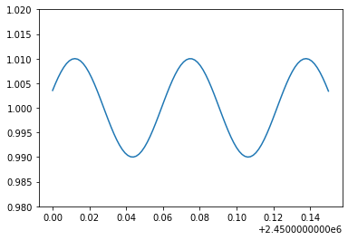
This might be the differential flux of a variable star. Let’s now simulate the fits images associated with the observation of this target:
[2]:
from prose.tutorials import simulate_observation

# so we have the same data
np.random.seed(40)

fits_folder = "./tutorial_dataset"
simulate_observation(time, target_dflux, fits_folder)
100%|██████████████████████████████████████████████████████████████████████████████████████████████| 100/100 [00:03<00:00, 32.95it/s]
here prose simulated comparison stars, their fluxes over time and some systematics noises.
Telescope setting#
We start by setting up the Telescope information we need for the reduction, for example some fits keywords that are specific to this observatory plus few specs:
[3]:
from prose import Telescope

_ = Telescope({
    "name": "A",
    "trimming": [40, 40],
    "pixel_scale": 0.66,
    "latlong": [31.2027, 7.8586],
    "keyword_light_images": "light"
})
Telescope 'a' saved
This has to be done only once and saves this telescope settings for any future use (whenever its name appears in fits headers). More details are given in the Telescope documentation.
Folder exploration#
The first thing we want to do is to see what is contained within our folder. For that we instantiate a FitsManager object on our folder to describe its content
[4]:
from prose import FitsManager

fm = FitsManager(fits_folder, depth=2)
fm
RUN Parsing FITS: 100%|█████████████████| 106/106 [00:00<00:00, 2226.95images/s]
[4]:
| date | telescope | filter | type | target | width | height | files | |
|---|---|---|---|---|---|---|---|---|
| id | ||||||||
| 3 | 2022-09-08 | A | bias | prose | 600 | 600 | 1 | |
| 4 | 2022-09-08 | A | dark | prose | 600 | 600 | 1 | |
| 2 | 2022-09-08 | A | a | flat | prose | 600 | 600 | 4 |
| 1 | 2022-09-08 | A | a | light | prose | 600 | 600 | 100 |
We have 100 images of the prose target together with some calibration files. More info about the FitsManager object here.
Choosing a reference image#
In order to perform the photometric extraction on all images, we will select a reference image
[5]:
from prose import Image

# image 0 will be our reference
ref = Image(fm.all_images[0])
and apply the following sequence to get the stars we want to perform photometry on
[6]:
from prose import Sequence, blocks

calibration = Sequence([
    blocks.Calibration(darks=fm.all_darks, bias=fm.all_bias, flats=fm.all_flats),
    blocks.Trim(),
    blocks.SegmentedPeaks(), # stars detection
    blocks.Cutouts(),                   # making stars cutouts
    blocks.MedianPSF(),                 # building PSF
    blocks.psf.Moffat2D(),              # modeling PSF
])

calibration.run(ref, show_progress=False)
ref.show()
INFO Building master bias
INFO Building master dark
INFO Building master flat
[6]:
<AxesSubplot:>
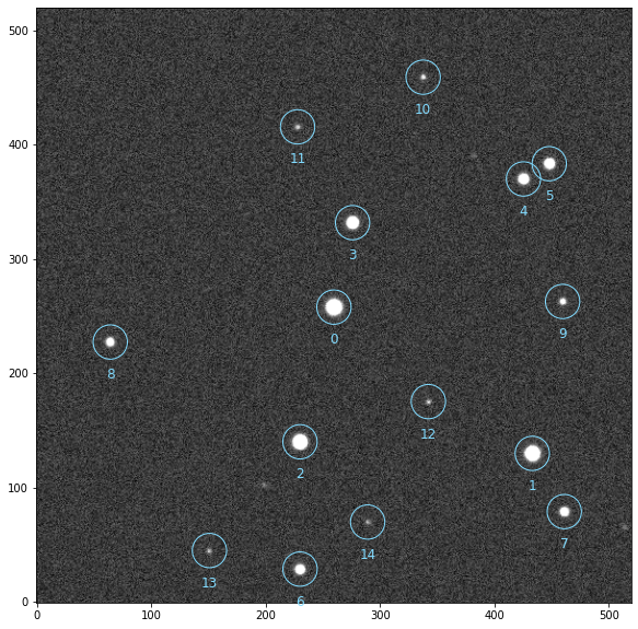
You can use a Gaia query to define which stars you want the photometry from (e.g. if too faint to be detected here)
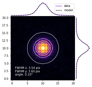
and here is the global PSF
[7]:
ref.plot_psf_model()
Photometry#
We can now extract the photometry of these stars
[8]:
photometry = Sequence([
    *calibration[0:-1],                   # apply the same calibration to all images
    blocks.psf.Moffat2D(reference=ref),   # providing a reference imporve the PSF optimisation
    blocks.detection.LimitStars(min=3),   # discard images not featuring enough stars
    blocks.Twirl(ref.stars_coords),       # compute image transformation

    # set stars to the reference ones and apply the inverse
    # transformation previously found to match the ones in the image
    blocks.Set(stars_coords=ref.stars_coords),
    blocks.AffineTransform(data=False, inverse=True),

    blocks.BalletCentroid(),                            # stars centroiding
    blocks.PhotutilsAperturePhotometry(scale=ref.fwhm), # aperture photometry
    blocks.Peaks(),

    # Retrieving data from images in a conveniant way (see later)
    blocks.XArray(
        ("time", "jd_utc"),
        ("time", "bjd_tdb"),
        ("time", "flip"),
        ("time", "fwhm"),
        ("time", "fwhmx"),
        ("time", "fwhmy"),
        ("time", "dx"),
        ("time", "dy"),
        ("time", "airmass"),
        ("time", "exposure"),
        ("time", "path"),
        ("time", "sky"),
        (("time", "apertures", "star"), "fluxes"),
        (("time", "apertures", "star"), "errors"),
        (("time", "apertures", "star"), "apertures_area"),
        (("time", "apertures", "star"), "apertures_radii"),
        (("time", "apertures"), "apertures_area"),
        (("time", "apertures"), "apertures_radii"),
        ("time", "annulus_rin"),
        ("time", "annulus_rout"),
        ("time", "annulus_area"),
        (("time", "star"), "peaks"),
        name="xarray"
    ),

    # Stack image
    blocks.AffineTransform(stars=False, data=True),
    blocks.Stack(ref, name="stack"),
])

photometry.run(fm.all_images)
RUN 100%|█████████████████████████████████| 100/100 [00:09<00:00, 10.06images/s]
All our data lie in the blocks.Xarray block, that we will transform into a convenient Observation object
[9]:
from prose import Observation

obs = Observation(photometry.xarray.to_observation(photometry.stack.stack, sequence=photometry))
INFO Time converted to BJD TDB
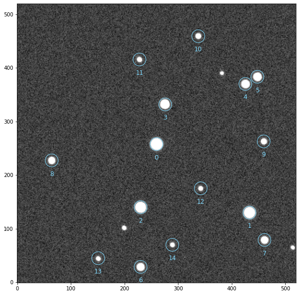
Photometry analysis#
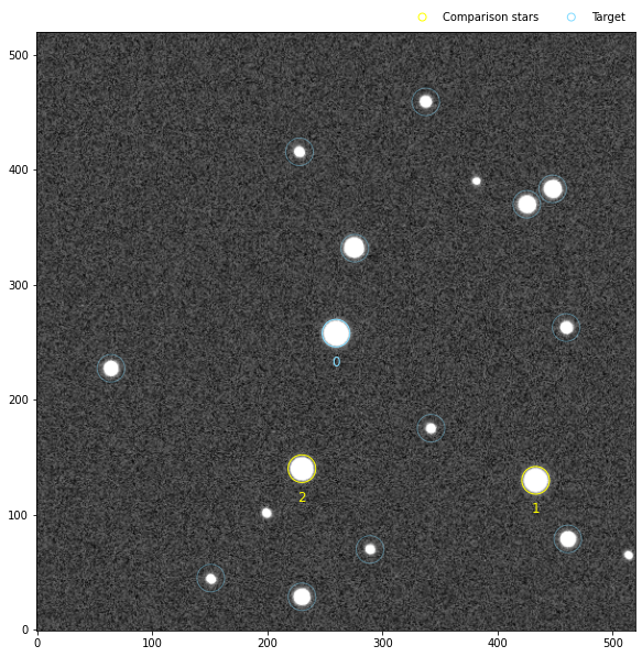
To show the stack image of the observation and see what obs contains:
[10]:
obs.show_stars(size=8)
[11]:
obs
[11]:
<xarray.Dataset>
Dimensions:          (time: 100, apertures: 32, star: 15, w: 520, h: 520, n: 2)
Coordinates:
    stack            (w, h) float64 299.5 300.4 300.9 ... 300.8 301.6 300.2
  * time             (time) float64 2.45e+06 2.45e+06 ... 2.45e+06 2.45e+06
    stars            (star, n) float64 259.8 257.8 433.2 ... 44.97 289.2 69.88
Dimensions without coordinates: apertures, star, w, h, n
Data variables: (12/20)
    jd_utc           (time) float64 2.45e+06 2.45e+06 ... 2.45e+06 2.45e+06
    bjd_tdb          (time) float64 2.45e+06 2.45e+06 ... 2.45e+06 2.45e+06
    flip             (time) object None None None None ... None None None None
    fwhm             (time) float64 3.576 3.576 3.576 ... 3.576 3.576 3.576
    fwhmx            (time) float64 3.599 3.599 3.599 ... 3.599 3.599 3.599
    fwhmy            (time) float64 3.553 3.553 3.553 ... 3.553 3.553 3.553
    ...               ...
    apertures_area   (apertures, time) float64 0.3999 0.3999 ... 2.464e+03
    apertures_radii  (apertures, time) float64 0.3568 0.3568 ... 28.01 28.01
    annulus_rin      (time) float64 17.84 17.84 17.84 ... 17.84 17.84 17.84
    annulus_rout     (time) float64 28.54 28.54 28.54 ... 28.54 28.54 28.54
    annulus_area     (time) float64 1.56e+03 1.56e+03 ... 1.56e+03 1.56e+03
    peaks            (star, time) float64 5.909e+04 5.646e+04 ... 484.1 482.1
Attributes: (12/36)
    SIMPLE:       1
    BITPIX:       -64
    NAXIS:        2
    NAXIS1:       520
    NAXIS2:       520
    TELESCOP:     A
    ...           ...
    filter:       a
    exptime:      1
    name:         prose
    date:         2022-09-08
    time_format:  bjd_tdb
photometry: ['Calibration', 'Trim', 'SegmentedPeaks', 'Cutouts', 'Media...Note
More details on the structure of these data products (and the representation above) in data products description
If target was not specified in the reduction process, we need to specify it before producing our differential Photometry.
[12]:
obs.target = 0
obs.broeg2005()
obs.plot()
plt.ylim(0.98, 1.02)
[12]:
(0.98, 1.02)
Note
We could also have picked the comparison stars ourselves using diff from Observation
We used the Broeg 2005 algorithm to build the differential light-curve and ended by plotting it. We can check the comparison stars with
[13]:
obs.show_stars(size=8)
and continue with further visualisation or analysis. All available plotting and analysis methods are described in Observation.
To save your analysis into the same phot file
[14]:
obs.save(f"{obs.label}.phot")
INFO saved /Users/lgrcia/code/prose/docs/source/notebooks/A_20220908_prose_a.phot
Some more details#
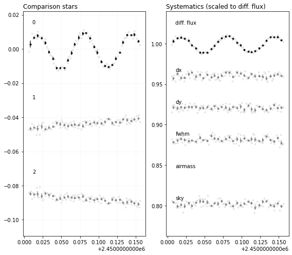
Observation plots#
From the Observation object many things can be plotted. For example here are the comparison light curves as well as the systematics data:
[16]:
plt.figure(figsize=(8, 7))

plt.subplot(121)
obs.plot_comps_lcs()

plt.subplot(122)
obs.plot_systematics()
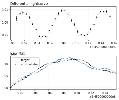
here is another useful one showing the raw fluxes as well as the artificial light curve (a weighted mean of the comparison stars - see Broeg 2005 paper)
[17]:
plt.figure(figsize=(6, 5))
obs.plot_raw_diff()
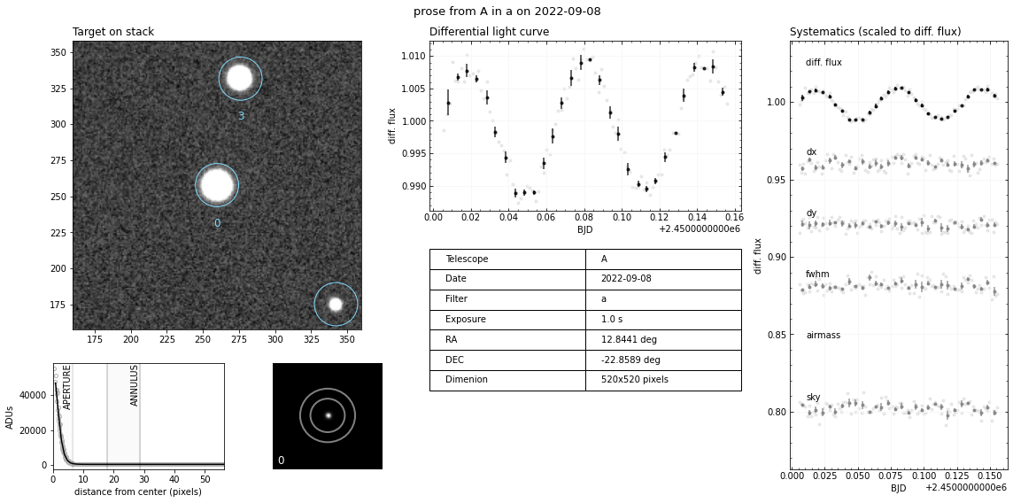
or a nice summary
[18]:
obs.plot_summary()
To see all possible plotting options check the Observation API