Hi’iaka occultation

Hiʻiaka is the largest, outer moon of the trans-Neptunian dwarf planet Haumea. We observed Hiʻiaka occulting a bright star, helping in the study of the moon’s orbital and physical parameters.

This observation was done with the 1-m telescope Artemis and consists of 1 s. short exposures, requiring images to be small in size (46x41 pixels to reduce the overhead time of the telescope). In this tutorial, we will extract the raw flux time-series of the star occulted by Hi’iaka.

Images

We start by scanning our dataset

from prose import FitsManager, utils

fm = FitsManager("/Users/lgrcia/data/Hiaka_occultation_20220609_Artemis", depth=1)
fm.observations(hide_exposure=False)

RUN Parsing FITS:  47%|███████▉         | 263/561 [00:00<00:00, 1317.24images/s]

INFO telescope  not found - using default

RUN Parsing FITS: 100%|█████████████████| 561/561 [00:00<00:00, 1331.57images/s]

	date	telescope	filter	type	target	width	height	exposure	files
id
1	2022-06-09		Clear	light	2002MS4_Artemis_clear_2x2bin	46	41	1.0	556
2	2022-06-09			bias	2002MS4_Artemis_clear_2x2bin	46	41	0.0	5

For this observation we only have bias calibration images. We see that some images could not be recognized. To solve this problem we can define an Image loader with the telescope pre-defined

from prose import Image

loader = Image.from_telescope("Artemis")

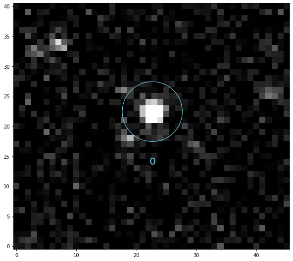
Reference

We then detect the stars for which the photomety will be extracted

from prose import Sequence, blocks, Image

images = fm.all_images
ref = loader(images[0])

calibration = Sequence([
    blocks.Calibration(bias=fm.all_bias, loader=loader),
    blocks.SegmentedPeaks(n_stars=1, auto=True)
])

calibration.run(ref, show_progress=False, loader=loader)
_ = ref.show(ms=5, fs=20, zscale=False)

INFO Building master bias
INFO No dark images set
INFO No flat images set

The reduction sequence

# to retrieve time and flux from images
data = blocks.Get("jd_utc", "fluxes")

reduction = Sequence([
    *calibration,
    blocks.Set(stars_coords=ref.stars_coords.copy()), # coordinates of the stars
    blocks.centroids.Quadratic(limit=4),
    blocks.PhotutilsAperturePhotometry(scale=False), # aperture photometry
    data
])

reduction.run(images, loader=loader)

RUN 100%|█████████████████████████████████| 556/556 [00:11<00:00, 49.02images/s]

we can now vizualise our light curve

import numpy as np
import matplotlib.pyplot as plt

time = np.array(data.jd_utc)
fluxes = np.array(data.fluxes) # shape is (time, apertures, stars)

# plotting aperture 10, star 0
flux = fluxes[:, 10, 0]
plt.plot(time - 2450000, flux, ".-", c="0.3")
_ = plt.xlim(9740.728, 9740.731)

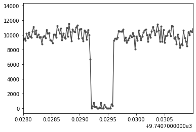
This is a full occultation that we should be able to see on the images directly!

Seeing the star disapear

In order to see the images as they are processed, we will use the blocks from the prose.blocks.vizualisation module. The PlotVideo block takes a plotting function as argument, which takes as input an Image object. Let’s implement it

def plot(image):
    plt.figure(None, (10,4))
    ax = plt.subplot(121, xlabel="JD-utc - 2450000", ylabel="diff. flux")
    time.append(image.jd_utc - 2450000)
    flux.append(image.fluxes[10,0]/10000)
    ax.plot(time, flux, ".-", c="0.3")
    plt.xlim(9740.7285, 9740.7305)
    ax.set_ylim(-0.2, 1.3)
    ax.set_title(f"Artemis 2002MS4 occultation ({ref.date.date()})")
    ax2 = plt.subplot(122)
    image.show(zscale=False, ms=5, fs=20, ax=ax2)
    plt.tight_layout()

and use it within a sequence that also contain the photometric extraction blocks

# this is set in plot
time = []; flux = []

viz = Sequence([
    *reduction,
    blocks.vizualisation.PlotVideo(plot, "static/hiaka.gif", fps=17)
])

# Only the images close to the occultation
viz.run(images[191:260], loader=loader)

RUN 100%|███████████████████████████████████| 69/69 [00:06<00:00, 10.34images/s]

Here is the movie.gif where we indeed see the star being occulted

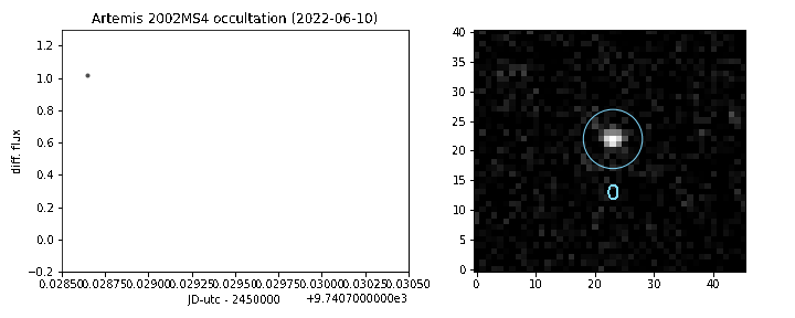
Note

Setting limit=3 in Quadratic allows to keep the aperture fixed when the star’s centroid is farther than limit pixel away from the initial position (we see that on the video when the star is occulted)