Catalogs & Plate solving#
It is often required to match your detected stars with a catalog. Let’s load an example image (from an archive like SDSS) and see how to do that
[1]:
from prose.archive import sdss_image
[2]:
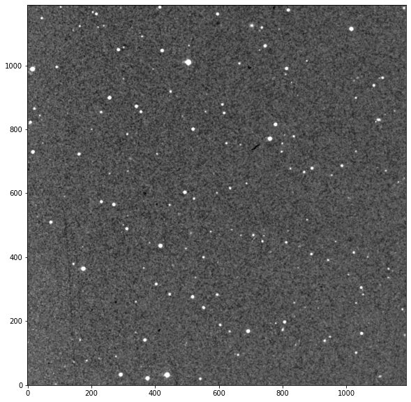
# an image of TRAPPIST-1
image = sdss_image(("23 06 29.3684", "-05 02 29.0373"), (20, 20))
image.show()
INFO Querying https://archive.stsci.edu/cgi-bin/dss_form
[2]:
<AxesSubplot:>
In our case, the image is plate solved, we can check with
[3]:
image.plate_solved
[3]:
True
Querying a catalog#
To query a catalog we can use a catalog block from the prose.blocks.catalogs module
[4]:
from prose.blocks import catalogs
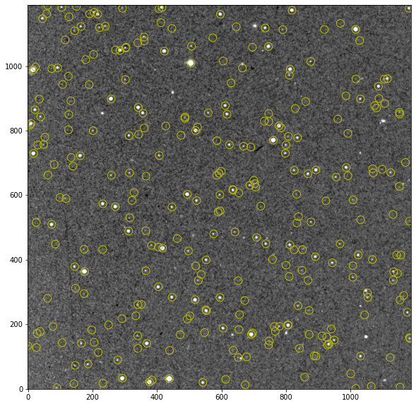
image = catalogs.GaiaCatalog(mode="replace")(image)
# visualizing the catalog stars
image.show(stars=False)
image.plot_catalog("gaia")
An overlay with labels can be plotted with
[5]:
image.show_cutout(star=(400,500), size=300)
image.plot_catalog("gaia", label=True, color="w")
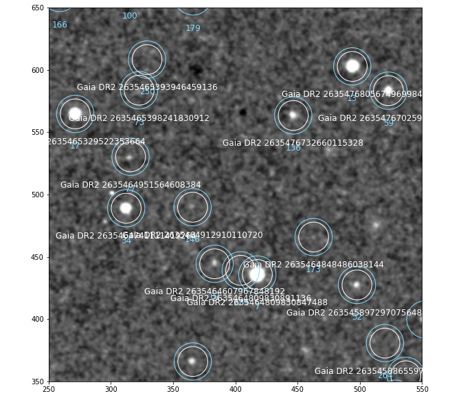
We see here that the stars_coords (plotted by default with image.show_cutout) are set to the queried stars
Note
If instead you want to cross-match the queried stars to already existing Image.stars_coords, use catalogs.GaiaCatalog(mode=crossmatch). This way the index of the star in stars_coords is the same as the index in the catalog (see the dataframe below)
The full catalogs can be found at
[6]:
image.catalogs["gaia"]
[6]:
| index | solution_id | id | source_id | random_index | ref_epoch | ra | ra_error | dec | dec_error | ... | flame_flags | radius_val | radius_percentile_lower | radius_percentile_upper | lum_val | lum_percentile_lower | lum_percentile_upper | datalink_url | x | y | |
|---|---|---|---|---|---|---|---|---|---|---|---|---|---|---|---|---|---|---|---|---|---|
| 0 | 3 | 1635721458409799680 | Gaia DR2 2635480237353372160 | 2635480237353372160 | 1145454718 | 2015.5 | 346.646498 | 0.038742 | -4.925421 | 0.032160 | ... | 200111 | 1.664209 | 1.603750 | 1.729316 | 3.345175 | 3.252988 | 3.437362 | https://gea.esac.esa.int/data-server/datalink/... | 505.175805 | 1009.615838 |
| 1 | 5 | 1635721458409799680 | Gaia DR2 2635456945746189696 | 2635456945746189696 | 817258039 | 2015.5 | 346.666253 | 0.037022 | -5.199083 | 0.039163 | ... | 200111 | 1.103787 | 0.998070 | 1.129748 | 1.315697 | 1.285068 | 1.346326 | https://gea.esac.esa.int/data-server/datalink/... | 438.452400 | 31.418957 |
| 2 | 6 | 1635721458409799680 | Gaia DR2 2635479550158605056 | 2635479550158605056 | 132373045 | 2015.5 | 346.784044 | 0.044148 | -4.930801 | 0.048522 | ... | 200111 | 2.737030 | 2.628122 | 2.930485 | 3.735508 | 3.536159 | 3.934858 | https://gea.esac.esa.int/data-server/datalink/... | 16.542186 | 988.603203 |
| 3 | 9 | 1635721458409799680 | Gaia DR2 2635478076985292160 | 2635478076985292160 | 1431076968 | 2015.5 | 346.574810 | 0.026821 | -4.992565 | 0.019001 | ... | 200111 | 6.997863 | 6.758047 | 7.126602 | 27.008816 | 22.342409 | 31.675222 | https://gea.esac.esa.int/data-server/datalink/... | 760.686001 | 770.568960 |
| 4 | 15 | 1635721458409799680 | Gaia DR2 2635463852053602176 | 2635463852053602176 | 1437357409 | 2015.5 | 346.739864 | 0.025791 | -5.105819 | 0.025741 | ... | 200111 | 1.229900 | 1.099773 | 1.576203 | 1.411291 | 1.334785 | 1.487797 | https://gea.esac.esa.int/data-server/datalink/... | 175.786311 | 363.737573 |
| ... | ... | ... | ... | ... | ... | ... | ... | ... | ... | ... | ... | ... | ... | ... | ... | ... | ... | ... | ... | ... | ... |
| 297 | 535 | 1635721458409799680 | Gaia DR2 2635481165066395776 | 2635481165066395776 | 1069485838 | 2015.5 | 346.578783 | 1.212314 | -4.969499 | 1.012364 | ... | <NA> | NaN | NaN | NaN | NaN | NaN | NaN | https://gea.esac.esa.int/data-server/datalink/... | 746.294694 | 852.943247 |
| 298 | 544 | 1635721458409799680 | Gaia DR2 2635457525566337664 | 2635457525566337664 | 949993158 | 2015.5 | 346.719172 | 1.193311 | -5.152310 | 1.296831 | ... | <NA> | NaN | NaN | NaN | NaN | NaN | NaN | https://gea.esac.esa.int/data-server/datalink/... | 249.894255 | 197.870557 |
| 299 | 554 | 1635721458409799680 | Gaia DR2 2635479618878183680 | 2635479618878183680 | 688393043 | 2015.5 | 346.753414 | 1.898055 | -4.936480 | 2.364617 | ... | <NA> | NaN | NaN | NaN | NaN | NaN | NaN | https://gea.esac.esa.int/data-server/datalink/... | 125.443276 | 968.715832 |
| 300 | 566 | 1635721458409799680 | Gaia DR2 2635467111934793088 | 2635467111934793088 | 515167063 | 2015.5 | 346.774041 | 1.456007 | -4.989243 | 1.606014 | ... | <NA> | NaN | NaN | NaN | NaN | NaN | NaN | https://gea.esac.esa.int/data-server/datalink/... | 52.846621 | 779.881605 |
| 301 | 574 | 1635721458409799680 | Gaia DR2 2635460136906448768 | 2635460136906448768 | 78090585 | 2015.5 | 346.782185 | 1.561662 | -5.171663 | 1.500308 | ... | <NA> | NaN | NaN | NaN | NaN | NaN | NaN | https://gea.esac.esa.int/data-server/datalink/... | 26.350389 | 127.863674 |
302 rows × 98 columns
Plate solving#
To plate solve an image we can use the following sequence
[7]:
from prose import Sequence, blocks

plate = Sequence([
    blocks.detection.SegmentedPeaks(min_separation=15, n_stars=15),
    blocks.catalogs.PlateSolve(debug=True)
])

plate.run(image, show_progress=False)
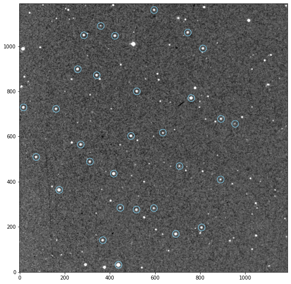
Seeing the markers on the stars (only with debug=True) in the image shows that the plate solving was successful
Note
PlateSolve is slow so it is not recomanded to use this block in a sequence with more than 5 images. Instead you can pass a plate-solved ref_image to this block so that catalog stars are queried only once