Modeling#
prose does not implement a modeling framework, many options are currently available in python. However, it features some tools to aid in selecting the right model, mainly linear ones.
In this tutorial we will review some of these tools and show how the prose products can conveniently be used within exoplanet, itself using the pymc3 inference framework.
Tutorial requirements:
<li>exoplanet</li>
<li>pymc3_ext</li>
<li>corner</li>
Making up some data#
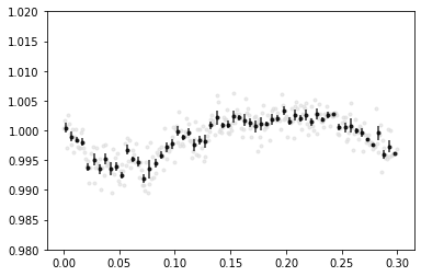
As usual we will work on synthetic data. Here we propose to analyse a planetary transit light curve in which we added some instrumental signals:
[1]:
import numpy as np
import matplotlib.pyplot as plt
from prose.simulations import observation_to_model

np.random.seed(37)

time = np.linspace(0, 0.3, 300)
obs = observation_to_model(time)
obs.plot()
_ = plt.ylim(0.98, 1.02)
INFO Could not convert time to BJD TDB
Note
In what follows we will consider that we already have a good knowledge of our transit parameters. This is for the tutorial’s purpose and one can adapt it by adjusting the model’s priors (especially in the inference part).
Linear models#
Polynomial systematics#
It is common to model the instrumental signals using a linear model involving some systematic measurements. Let’s say that we measured an explanatory variable \(\boldsymbol{x}\) along time (the temperature of the detector for example). If \(\boldsymbol{f}\) is our measured flux sampled along the same time, we can suppose that it can be modeled as a polynomial order 2 of \(\boldsymbol{x}\) plus some gaussian noise, so that:
\(a\), \(b\), \(c\) being free parameters. This can be writen in the matrix form:
with \(X\) the design matrix. \(X\) is known so that this linear equation can be solved for \(w\) through ordinary least square. Before doing any of that let’s make sure our observation is clean
[2]:
# removing obvious outlier
obs = obs.sigma_clip()
We can now use prose methods to build a linear model by defining its design matrix \(X\). Here we decided to set an order 2 polynomial of the sky data to start with
[3]:
from prose import models
import matplotlib.pyplot as plt

X = models.polynomial(obs.sky, 2)

trend = obs.lstsq(X)

obs.plot()
plt.plot(obs.time, trend)
_ = plt.ylim(0.98, 1.02)
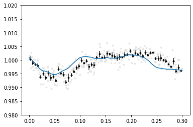
Although it’s not very good, the model is certainly not complete. Let’s make it better.
Adding a transit#
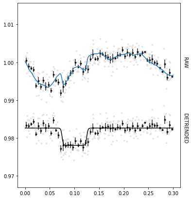
Our data contain a transit signal which, at first order, can be modeled as a scaled transit of unitary depth. To do that we will add this template to our design matrix. Here, we will use the more conveniant Observation.polynomial() method which comes handy for more complex models.
[4]:
import numpy as np

t0 = 0.1
duration = 0.05

X = np.hstack([
    obs.polynomial(sky=1, dy=1),
    obs.transit(t0, duration)
])

# Notice the use of split to get the transit model
trend, transit = obs.lstsq(X, split=-1)
[5]:
from prose import viz

viz.plot_systematics_signal(obs.time, obs.diff_flux, trend, transit)
Model selection#
In the last sections we used arbitrary models of the systematics. It seems the last one is complete and not too complex but wiser choice can be made using model selection crtieria like BIC or AIC. Here we will iterate on a range of possible models and compute which one gives the best BIC:
[6]:
# we authorize combinations up to order 5

best = obs.best_polynomial(sky=5, dy=5, add=obs.transit(t0, duration))
print("best model:", best)
best model: {'sky': 1, 'dy': 2}
This confirms our previous guess. This order combination can be used within the next step to do a proper modeling. Before doing that let see what is the preferred model without a transit:
[7]:
best_no_transit = obs.best_polynomial(sky=5, dy=5)
print("best orders:", best_no_transit)

another_trend = obs.polynomial(**best_no_transit)
best_trend = obs.polynomial(**best)

obs.plot()
plt.plot(obs.time, obs.lstsq(another_trend), label="another")
plt.plot(obs.time, obs.lstsq(best_trend), c="C3", label="best")
plt.ylim(0.98, 1.02); _ = plt.legend()
best orders: {'sky': 1, 'dy': 5}
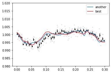
This was just for fun and shows that adding dy order 5 favors the fit while keeping the model simple. We notice that this estimate naturraly depends on how complete the model is (here not complete due to the transit missing).
Bayesian modeling#
We will now use exoplanet to infer of our transit parameters. For this part of the tutorial you will need exoplanet and corner to be installed.
[8]:
# we use the best order combination found in the previous section

X = obs.polynomial(**best)
The basic principle of pymc3 is to let you define free parameters distributions and specify the models which depend on them before doing any computation. Doing so, a pre-optimized graph is built once making any later execution much faster. This comes handy for inference since a lot of samples need to be drawn from your posterior distribution. Let’s build our pymc3 model with exoplanet (lot more details here):
[9]:
# here we use exoplanet 0.5.2

import pymc3 as pm
import pymc3_ext as pmx
import exoplanet as xo
from prose.utils import earth2sun

with pm.Model() as model:

    # Transit parameters
    # ------------------
    period = pm.Uniform("period", 0.1, 3)
    r = pm.Uniform("r", 3, 8)*earth2sun
    w = pm.Flat("s", len(X.T), testval=np.linalg.lstsq(X, obs.diff_flux, rcond=None)[0])

    # Keplerian orbit
    # ---------------
    orbit = xo.orbits.KeplerianOrbit(period=period, t0=0.1)
    # starry light-curve
    light_curves = xo.LimbDarkLightCurve([0.1, 0.4]).get_light_curve(orbit=orbit, r=r, t=obs.time)
    transit = pm.Deterministic("transit", pm.math.sum(light_curves, axis=-1))

    # Systematics and final model
    # ---------------------------
    systematics = X@w
    mu = pm.Deterministic("mu", transit + systematics)

    # Likelihood
    # ----------
    pm.Normal("obs", mu=mu, sd=obs.diff_error, observed=obs.diff_flux)

    # Maximum a posteriori
    # --------------------
    opt = pmx.optimize(start=model.test_point)
WARNING (theano.link.c.cmodule): install mkl with `conda install mkl-service`: No module named 'mkl'
optimizing logp for variables: [s, r, period]
message: Optimization terminated successfully.
logp: 1380.7241856821806 -> 1448.2841596009973
We can plot the maximum a posteriori which will be the starting point of our sampling algorithm
[10]:
obs.plot()
plt.plot(obs.time, opt["mu"], label="MAP")
plt.plot(obs.time, opt["transit"]+1, "--", color="0.5", label="transit")
plt.ylim(0.98, 1.02)
plt.title("Maximum a posteriori", loc="left")
_ = plt.legend()
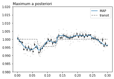
Not bad. Let’s sample the posterior likelihood
[11]:
np.random.seed(42)

with model:
    trace = pm.sample(
        tune=2000,
        draws=2000,
        initvals=opt,
        cores=2,
        chains=2,
        init="adapt_full",
        target_accept=0.9,
        return_inferencedata=False
    )
Auto-assigning NUTS sampler...
Initializing NUTS using adapt_full...
/opt/homebrew/Caskroom/miniforge/base/envs/prose/lib/python3.9/site-packages/pymc3/step_methods/hmc/quadpotential.py:510: UserWarning: QuadPotentialFullAdapt is an experimental feature
  warnings.warn("QuadPotentialFullAdapt is an experimental feature")
Multiprocess sampling (2 chains in 2 jobs)
NUTS: [s, r, period]
/opt/homebrew/Caskroom/miniforge/base/envs/prose/lib/python3.9/site-packages/scipy/stats/_continuous_distns.py:624: RuntimeWarning: overflow encountered in _beta_ppf
  return _boost._beta_ppf(q, a, b)
/opt/homebrew/Caskroom/miniforge/base/envs/prose/lib/python3.9/site-packages/scipy/stats/_continuous_distns.py:624: RuntimeWarning: overflow encountered in _beta_ppf
  return _boost._beta_ppf(q, a, b)
Sampling 2 chains for 2_000 tune and 2_000 draw iterations (4_000 + 4_000 draws total) took 10 seconds.
We can now make a corner plot of the parameters of interest. We marked in blue the true values used to generate our synthetic data.
[12]:
import corner

samples = pm.trace_to_dataframe(trace, varnames=["period", "r"])
_ = corner.corner(samples, truths=[0.6, 7.])
WARNING:root:Pandas support in corner is deprecated; use ArviZ directly
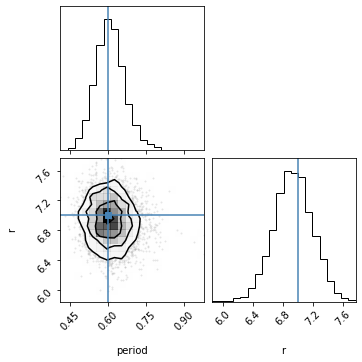
Quite close! Again, our priors are not realistic and inferring the parameters of a real unknown transit will require some adjustments.
Recomendations#
We highly recomand the use of the excellent exoplanet (and starry for more speific needs) packages and documentations. To see if they fit your needs, the case studies pages of exoplanet is a good place to start.