Exoplanet transit

In this tutorial we will reduce raw images to produce a transit light curve of WAPS-12 b. All images can be downloaded from https://astrodennis.com/.

Managing the FITS

For this observation, the headers of the calibration images do not contain information about the nature of each image, bias, dark or flat. We will then retrieve our images by hand (where usually we would employ a FitsManager object)

from glob import glob
from pathlib import Path

folder = Path("/Users/lgarcia/data/wasp12_example_dataset")

darks = glob(str(folder / "Darks/*.fit"))
bias = glob(str(folder / "Bias/*.fit"))
flats = glob(str(folder / "Flats/*.fit"))
sciences = sorted(glob(str(folder / "ScienceImages/*.fit")))

The full reduction

What follows is the full reduction sequences, including the selection of a reference image to align sources and scale apertures on. More details are provided in the basic Photometry tutorial

import numpy as np
from prose import FITSImage, Sequence, blocks

# reference is middle image
ref = FITSImage(sciences[len(sciences) // 2])

calibration = Sequence(
    [
        blocks.Calibration(darks=darks, bias=bias, flats=flats),
        blocks.Trim(),
        blocks.PointSourceDetection(n=40),  # stars detection
        blocks.Cutouts(21),  # stars cutouts
        blocks.MedianEPSF(),  # building EPSF
        blocks.psf.Moffat2D(),  # modeling EPSF
    ]
)

calibration.run(ref, show_progress=False)

photometry = Sequence(
    [
        calibration[0],  # calibration block (same as above)
        blocks.PointSourceDetection(n=12, minor_length=8),  # fewer stars detection
        blocks.Cutouts(21),  # stars cutouts
        blocks.MedianEPSF(),  # building EPSF
        blocks.Gaussian2D(ref),  # modeling EPSF with initial guess
        blocks.ComputeTransformTwirl(ref),  # compute alignment
        blocks.AlignReferenceSources(ref),  # alignment
        blocks.CentroidQuadratic(),  # centroiding
        blocks.AperturePhotometry(),  # aperture photometry
        blocks.AnnulusBackground(),  # annulus background
        blocks.GetFluxes(
            "fwhm",
            airmass=lambda im: im.header["AIRMASS"],
            dx=lambda im: im.transform.translation[0],
            dy=lambda im: im.transform.translation[1],
        ),
    ]
)

photometry.run(sciences)

Warning

For image alignment only n=12 sources are being detected, but note that these sources are not the ones for which the photometry is extracted. Indeed, the following block AlignReferenceSources(ref) modifies the sources from each image, setting them to the sources of the references but aligned to each image.

We can check the total processing time of each block with

photometry

╒═════════╤════════╤═══════════════════════╤════════════════╕
│   index │ name   │ type                  │ processing     │
╞═════════╪════════╪═══════════════════════╪════════════════╡
│       0 │        │ Calibration           │ 1.755 s (4%)   │
├─────────┼────────┼───────────────────────┼────────────────┤
│       1 │        │ PointSourceDetection  │ 18.141 s (41%) │
├─────────┼────────┼───────────────────────┼────────────────┤
│       2 │        │ Cutouts               │ 2.075 s (5%)   │
├─────────┼────────┼───────────────────────┼────────────────┤
│       3 │        │ MedianEPSF            │ 0.165 s (0%)   │
├─────────┼────────┼───────────────────────┼────────────────┤
│       4 │        │ Gaussian2D            │ 2.907 s (7%)   │
├─────────┼────────┼───────────────────────┼────────────────┤
│       5 │        │ ComputeTransformTwirl │ 0.494 s (1%)   │
├─────────┼────────┼───────────────────────┼────────────────┤
│       6 │        │ AlignReferenceSources │ 0.125 s (0%)   │
├─────────┼────────┼───────────────────────┼────────────────┤
│       7 │        │ CentroidQuadratic     │ 1.312 s (3%)   │
├─────────┼────────┼───────────────────────┼────────────────┤
│       8 │        │ AperturePhotometry    │ 12.040 s (27%) │
├─────────┼────────┼───────────────────────┼────────────────┤
│       9 │        │ AnnulusBackground     │ 5.607 s (13%)  │
├─────────┼────────┼───────────────────────┼────────────────┤
│      10 │        │ GetFluxes             │ 0.024 s (0%)   │
╘═════════╧════════╧═══════════════════════╧════════════════╛

Differential photometry

Now that the photometry has been extracted, let’s focus on our target and produce a differential light curve for it.

All fluxes have been saved in the GetFluxes block, in a Fluxes object

from prose import Fluxes

fluxes: Fluxes = photometry[-1].fluxes

We can check the reference image, on which all images sources have been aligned, and pick our target

ref.show()

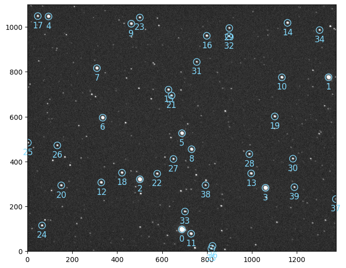
set this target (source 6) in the Fluxes object and proceed with automatic differential photometry

import matplotlib.pyplot as plt

fluxes.target = 6

# a bit of cleaning
nan_stars = np.any(np.isnan(fluxes.fluxes), axis=(0, 2)) # stars with nan fluxes
fluxes = fluxes.mask_stars(~nan_stars) # mask nans stars
fluxes = fluxes.sigma_clipping_data(bkg=3, fwhm=3) # sigma clipping

# differential photometry
diff = fluxes.autodiff()

# plotting
ax = plt.subplot(xlabel="time (JD)", ylabel="diff. flux", ylim=(0.94, 1.06))
diff.plot()
diff.bin(5 / 60 / 24, estimate_error=True).errorbar()

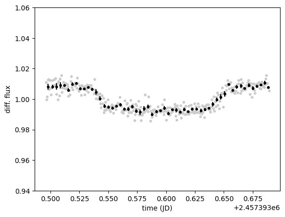
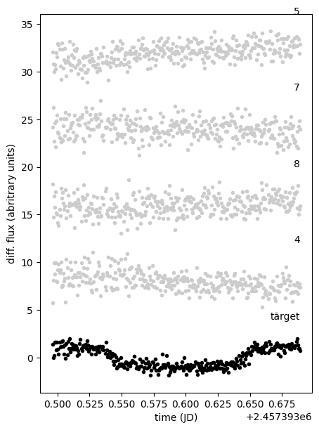
And here is our planetary transit. To validate the differential photometry and the automatic choice of comparison stars, we can plot their light curves along the target light curve

plt.figure(None, (5, 7))
ax = plt.subplot(xlabel="time (JD)", ylabel="diff. flux (abritrary units)")


# plotting only the first five comparisons
for j, i in enumerate([diff.target, *diff.comparisons[0:5]]):
    y = diff.fluxes[diff.aperture, i].copy()
    y = (y - np.mean(y)) / np.std(y) + 8 * j
    plt.text(
        diff.time.max(), np.mean(y) + 4, i if i != diff.target else "target", ha="right"
    )
    plt.plot(diff.time, y, ".", c="0.8" if i != diff.target else "k")

Explanatory measurements

To help modeling the light curve, some explanatory measurements have been stored in

diff.dataframe

	bkg	airmass	dx	dy	fwhm	time	flux
0	261.908217	1.878414	-0.314490	0.566460	4.823861	2.457393e+06	1.011125
1	263.309778	1.870291	-1.088033	0.466066	4.473168	2.457393e+06	0.999756
2	261.167119	1.862163	-0.868474	0.423316	4.369253	2.457393e+06	1.001618
3	252.933837	1.854302	-0.953985	0.551378	4.677914	2.457393e+06	1.012742
4	252.841623	1.846374	-1.025708	0.448884	4.735902	2.457393e+06	1.012824
...	...	...	...	...	...	...	...
327	157.205167	1.013443	1.007175	0.613441	4.130921	2.457394e+06	1.015685
328	157.248958	1.013356	1.577194	0.623359	4.012928	2.457394e+06	1.010365
329	156.650647	1.013278	0.737424	0.519273	4.491135	2.457394e+06	1.007430
330	156.423297	1.013210	0.700936	0.711975	4.576204	2.457394e+06	1.007304
331	157.131704	1.013150	0.977755	0.784270	4.015622	2.457394e+06	1.005600

332 rows × 7 columns

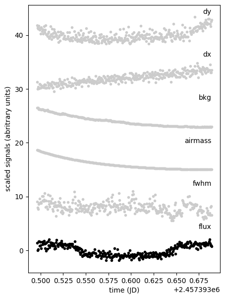
that we can plot to check for any correlation with the differential flux

plt.figure(None, (5, 7))
ax = plt.subplot(xlabel="time (JD)", ylabel="scaled signals (abritrary units)")

for i, name in enumerate(["flux", "fwhm", "airmass", "bkg", "dx", "dy"]):
    y = diff.df[name].copy()
    y = (y - np.mean(y)) / np.std(y) + 8 * i
    plt.text(diff.time.max(), np.mean(y) + 4, name, ha="right")
    plt.plot(diff.time, y, ".", c="0.8" if name != "flux" else "k")

Multiprocessing alternative

For those in a hurry, the photometry sequence can be made parallel

from prose.core.sequence import SequenceParallel

faster_photometry = SequenceParallel(
    [
        blocks.Calibration(darks=darks, bias=bias, flats=flats, shared=True),
        blocks.PointSourceDetection(
            n=12, minor_length=8
        ),  # stars detection for alignment
        blocks.Cutouts(21),  # stars cutouts
        blocks.MedianEPSF(),  # building EPSF
        blocks.Gaussian2D(ref),  # modeling EPSF with initial guess
        blocks.ComputeTransformTwirl(ref),  # compute alignment
        blocks.AlignReferenceSources(ref),  # align sources
        blocks.CentroidQuadratic(),  # centroiding
        blocks.AperturePhotometry(),  # aperture photometry
        blocks.AnnulusBackground(),  # annulus background
        blocks.Del("data", "sources", "cutouts"),  # (optional) reduce overhead
    ],
    [
        blocks.GetFluxes(
            "fwhm",
            airmass=lambda im: im.header["AIRMASS"],
            dx=lambda im: im.transform.translation[0],
            dy=lambda im: im.transform.translation[1],
        ),
    ],
)

faster_photometry.run(sciences)

The SequenceParallel class is a subclass of Sequence that allows to run blocks in parallel. This object takes two lists of blocks. The first sequence of blocks is run for each image on a different CPU core, the second is run sequentially and must contain all blocks that retain data and are slower to move between CPU cores.