Images photometry

After an observation is done, a common need is to reduce and extract fluxes from raw FITS images.

In this tutorial you will learn how to process a complete night of raw data from any telescope by building a data reduction Sequence with prose.

Simualting data

You can follow this tutorial on your own data or generate a synthetic dataset. As an example, let’s generate a light curve

import numpy as np
import matplotlib.pyplot as plt
from prose.simulations import simulate_observation

time = np.linspace(0, 0.15, 100) + 2450000
target_dflux = 1 + np.sin(time * 100) * 1e-2

plt.plot(time, target_dflux)
_ = plt.ylim(0.98, 1.02)

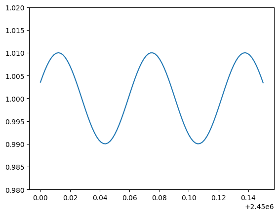
This might be the differential flux of a variable star. Let’s now simulate the fits images associated with the observation of this target:

# so we have the same data
np.random.seed(40)

fits_folder = "./tutorial_dataset"
simulate_observation(time, target_dflux, fits_folder)

100%|██████████| 100/100 [00:03<00:00, 31.43it/s]

here prose simulated comparison stars, their fluxes over time and some systematics noises.

Explore FITS

The first thing we want to do is to see what is contained within our folder. For that we instantiate a FitsManager object on our folder to describe its content

from prose import FitsManager

fm = FitsManager(fits_folder, depth=2)
fm

	date	telescope	filter	type	target	width	height	files
id
3	2023-04-19	A		bias	prose	600	600	1
4	2023-04-19	A		dark	prose	600	600	1
2	2023-04-19	A	a	flat	prose	600	600	4
1	2023-04-19	A	a	light	prose	600	600	100

We have 100 images of the prose target together with some calibration files.

Extracting photometry

Using a reference

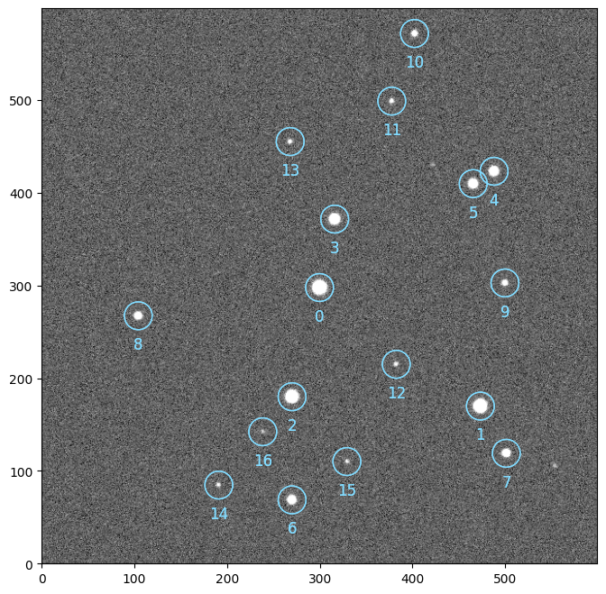
In order to perform the photometric extraction of stars fluxes on all images, we will select a reference image from which we will extract:

• The stars positions, then reused and detected on all images (after being aligned to the reference)

• The global full-width at half-maximum (fwhm) of the PSF, to scale the apertures used in the aperture photometry block

from prose import FITSImage

ref = FITSImage(fm.all_images[0])

Note

FITSImage is the primary function used to load a FITS image into an Image object. While other loaders wan be used, this loader is compatible with most of the images aquired from small to large-size ground based telescopes.

Let’s now build a Sequence to process the reference image

from prose import Sequence, blocks

calibration = Sequence(
    [
        blocks.Calibration(darks=fm.all_darks, bias=fm.all_bias, flats=fm.all_flats),
        blocks.Trim(),
        blocks.PointSourceDetection(),  # stars detection
        blocks.Cutouts(21),  # making stars cutouts
        blocks.MedianEPSF(),  # building PSF
        blocks.psf.Moffat2D(),  # modeling PSF
    ]
)

calibration.run(ref, show_progress=False)

ref.show()
ref.sources.plot()

Tip

You can use a Gaia query to define which stars you want the photometry from (e.g. if too faint to be detected here)

Aperture photometry

We can now extract the photometry of these stars

from astropy.stats import gaussian_sigma_to_fwhm

radii = np.linspace(0.2, 4, 30)

photometry = Sequence(
    [
        *calibration,  # calibration
        blocks.AlignReferenceSources(ref),  # alignment
        blocks.CentroidQuadratic(),  # centroiding
        blocks.AperturePhotometry(radii=radii),  # aperture photometry
        blocks.AnnulusBackground(),  # local background estimate
        blocks.GetFluxes(),
    ]
)

photometry.run(fm.all_images, loader=FITSImage)

Notice how we specified a loader to photometry.run, and instead of passing a list of Image objects, we passed a list of image paths. Although we cannot access each Image and its data individually, this allow to process a large amount of images without having to load them in memory. Instead, eadch image is loaded, processed and deleted in memory on the go.

The Fluxes object

The GetFluxes block provide a way to retrieve the fluxes computed by the AperturePhotometry minus the background estimated with AnnulusBackground

raw_fluxes = photometry[-1].fluxes

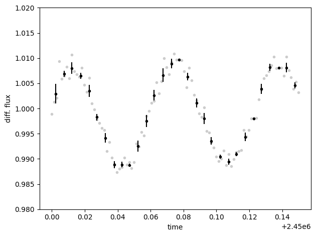
we can then produce the differential photometry with autodiff

# picking target
raw_fluxes.target = 0

# good practice
raw_fluxes = raw_fluxes.sigma_clipping_data(bkg=3)

# differential photometry
diff_fluxes = raw_fluxes.autodiff()
diff_fluxes.plot()
diff_fluxes.bin(0.005, True).errorbar()

plt.ylim(0.98, 1.02)
plt.xlabel("time")
plt.ylabel("diff. flux")
plt.tight_layout()

Show code cell content Hide code cell content

import shutil

shutil.rmtree(fits_folder)