Exoplanet transit

In this tutorial we will reduce raw images to produce a transit light curve of WAPS-12 b. All images can be downloaded from https://astrodennis.com/.

Managing the FITS

For this observation, the headers of the calibration images do not contain information about the nature of each image, bias, dark or flat. We will then retrieve our images by hand (where usually we would employ a FitsManager object)

from glob import glob

darks = glob("/Users/lgrcia/data/WASP12-astrodennis/Darks/*.fit")
bias = glob("/Users/lgrcia/data/WASP12-astrodennis/Bias/*.fit")
flats = glob("/Users/lgrcia/data/WASP12-astrodennis/Flats/*.fit")
sciences = sorted(glob("/Users/lgrcia/data/WASP12-astrodennis/ScienceImages/*.fit"))

The full reduction

wWhat follows is the full reduction sequences, including the selection of a reference image to align sources and scale apertures on. More details are provided in the basic Photometry tutorial

import numpy as np
from prose import FITSImage, Sequence, blocks

# reference is middle image
ref = FITSImage(sciences[len(sciences) // 2])

calibration = Sequence(
    [
        blocks.Calibration(darks=darks, bias=bias, flats=flats),
        blocks.Trim(),
        blocks.PointSourceDetection(n=20),  # stars detection
        blocks.Cutouts(21),  # stars cutouts
        blocks.MedianEPSF(),  # building EPSF
        blocks.psf.Moffat2D(),  # modeling EPSF
    ]
)

calibration.run(ref, show_progress=False)
radii = np.linspace(0.2, 8, 30)
calibration[2].n = 15  # only 15 stars for alignment

photometry = Sequence(
    [
        *calibration,  # calibration
        blocks.AlignReferenceSources(ref),  # alignment
        blocks.CentroidQuadratic(),  # centroiding
        blocks.AperturePhotometry(radii=radii),  # aperture photometry
        blocks.AnnulusBackground(),
        blocks.GetFluxes("fwhm", "keyword:AIRMASS"),
    ]
)

photometry.run(sciences)

Differential photometry

Now that the photometry has been extracted, let’s focus on our target and produce a differential light curve for it.

All fluxes have been saved in the GetFluxes block, in a Fluxes object

fluxes = photometry[-1].fluxes

We can check the reference image, on which all images sources have been aligned, and pick our target

ref.show()

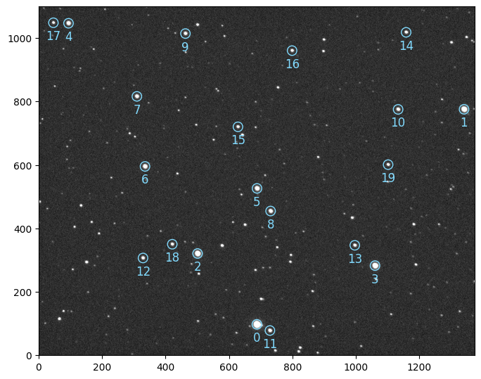
set this target (source 6) in the Fluxes object and proceed with automatic differential photometry

import matplotlib.pyplot as plt

fluxes.target = 6
# good practice
fluxes = fluxes.sigma_clipping_data(bkg=3, fwhm=3)
diff = fluxes.autodiff()

# plotting
ax = plt.subplot(xlabel="time (JD)", ylabel="diff. flux", ylim=(0.94, 1.06))
diff.plot()

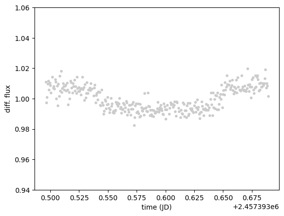
And here is our planetary transit. To help modeling the light curve, some explanatory measurements have been stored in

diff.dataframe

	bkg	fwhm	airmass	time	flux
0	250.263007	12.541211	1.878414	2.457393e+06	1.011166
1	262.606836	10.475859	1.870291	2.457393e+06	0.997370
2	261.537405	9.742434	1.862163	2.457393e+06	1.001082
3	252.502503	10.533297	1.854302	2.457393e+06	1.009875
4	241.739840	11.893354	1.846374	2.457393e+06	1.011724
...	...	...	...	...	...
320	149.832278	13.121772	1.013443	2.457394e+06	1.019027
321	157.090671	10.308623	1.013356	2.457394e+06	1.006965
322	149.277353	13.248450	1.013278	2.457394e+06	1.010045
323	148.409886	14.532337	1.013210	2.457394e+06	1.008293
324	155.043110	11.076587	1.013150	2.457394e+06	1.001656

325 rows × 5 columns