Quickstart

prose contains the structure to build astronomical images pipelines.

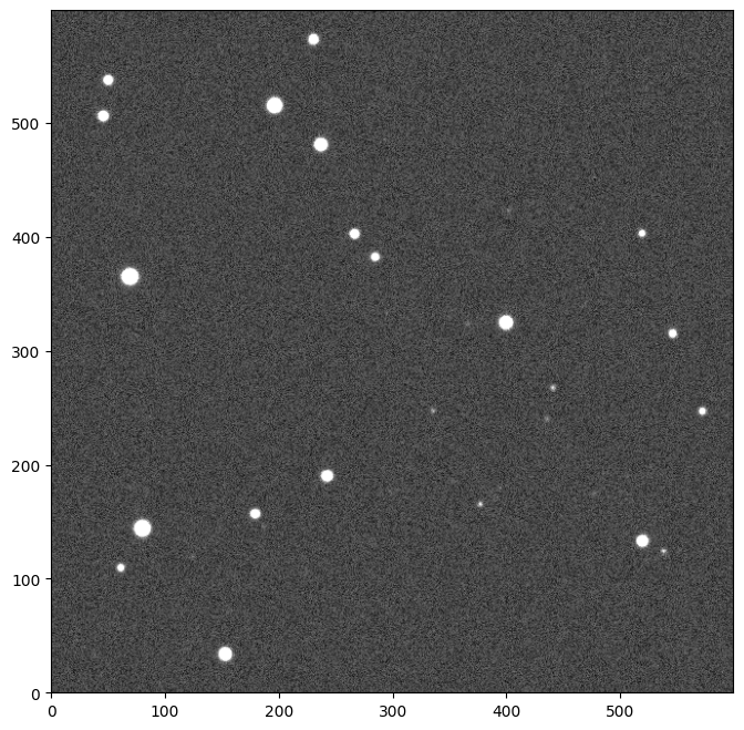
Here is a quick example pipeline to characterize the point spread function (PSF) of an image. Let’s start by loading an example Image.

from prose import Sequence, blocks, example_image
import matplotlib.pyplot as plt

# getting the example image
image = example_image()
image.show()

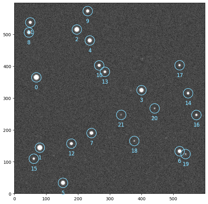
We can now build a Sequence containing single processing units called Block that will sequentially process our image.

sequence = Sequence(
    [
        blocks.detection.PointSourceDetection(),  # stars detection
        blocks.Cutouts(21),  # cutouts extraction
        blocks.MedianEPSF(),  # PSF building
        blocks.Moffat2D(),  # PSF modeling
    ]
)

sequence.run([image])

# plotting the detected stars
image.show()
image.sources.plot()

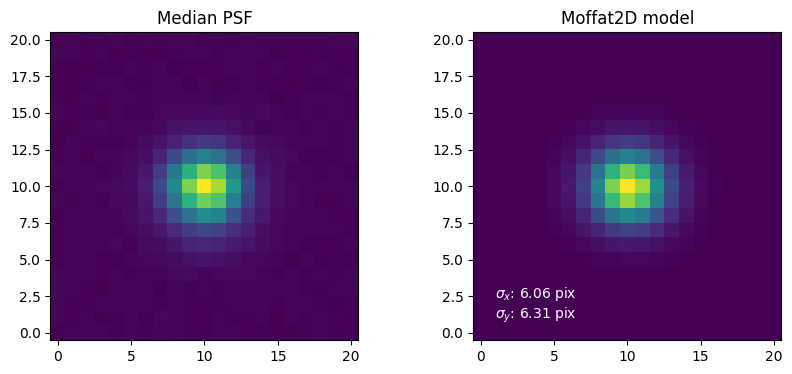
Let’s plot the results of the PSF building and modeling from the Image attributes.

plt.figure(None, (10, 4))

# PSF building
plt.subplot(1, 2, 1, title="Median PSF")
plt.imshow(image.epsf.data, origin="lower")

# PSF modeling
params = image.epsf.params
model = image.epsf.model

plt.subplot(1, 2, 2, title=f"Moffat2D model")
plt.imshow(model(params), origin="lower")
_ = plt.text(
    1,
    1,
    f"$\sigma_x$: {params['sigma_x']:.2f} pix\n$\sigma_y$: {params['sigma_y']:.2f} pix",
    c="w",
)

prose contains a wide variety of blocks implementing methods and algorithms commonly used in astronomical image processing.